Inferential statistics is a branch of statistics that allows us to make inferences or draw conclusions about a population based on a sample of data. It involves various methods and tests, each designed for specific types of data and research questions. In this article, we will explore what is inferential statistics and different types of inferential statistics, including hypothesis testing and regression analysis.
What is Inferential Statistics?
Let’s explore the concept of inferential statistics from different writers’ perspectives.
1. Authoritative Perspective: “Inferential statistics is the branch of statistics that enables us to draw conclusions and make predictions about a population based on a sample of data. It serves as the bridge between observed data and the larger context of the population. Inferential statistics involves a wide array of techniques, such as hypothesis testing, confidence intervals, and regression analysis, that provide the means to uncover patterns, relationships, and differences in data, making it an indispensable tool for scientific research and decision-making” (OpenStax College, 2014).
2. Scholarly Perspective: “Inferential statistics is the core of statistical inference, playing a pivotal role in scientific research. By leveraging probability theory and mathematical models, inferential statistics allows researchers to make generalizations about populations based on samples. It is the vehicle through which researchers test hypotheses, determine the significance of findings, and assess the reliability of observed relationships. Inferential statistics equips us with the tools to derive meaningful insights from data, enhancing the scientific method’s ability to draw substantive conclusions from limited information” (Moore, McCabe, & Craig, 2016).
3. Practical Perspective: “Inferential statistics is the practical arm of statistics, giving us the power to make informed decisions in real-world scenarios. It’s not just about numbers; it’s about making sense of data and applying it to solve problems. When you read market research, medical studies, or political polls, you are encountering the fruits of inferential statistics. It helps businesses make data-driven decisions, doctors tailor treatments, and policymakers create effective strategies. In essence, inferential statistics transforms raw data into actionable knowledge” (Trochim & Donnelly, 2008).
4. Data Scientist’s Perspective: “Inferential statistics is the compass that guides data scientists through the vast sea of data. It allows us to navigate uncertainty, answer questions, and make predictions. By sampling data, developing models, and calculating probabilities, we can unravel hidden insights and extract meaningful information. Whether it’s predicting customer behavior, optimizing algorithms, or understanding the impact of variables, inferential statistics is the tool that transforms data into actionable insights in the realm of data science” (McKinney, 2018).
Each perspective offers a unique angle on inferential statistics, highlighting its importance in different contexts, from scientific research to practical decision-making and data science. It’s a versatile and indispensable tool for anyone seeking to make sense of data and draw meaningful conclusions.
Different Types of Inferential Statistics:
Inferential statistics involves two main categories of techniques: hypothesis testing and regression analysis. Hypothesis testing is used to determine whether a specific hypothesis about a population parameter is supported by the sample data. On the other hand, regression analysis explores the relationships between variables, often involving the prediction of one variable based on one or more other variables.
1. Hypothesis Testing:
Hypothesis testing is a critical part of inferential statistics. It involves formulating a null hypothesis (H0) and an alternative hypothesis (Ha), collecting sample data, and then using statistical tests to determine whether the null hypothesis should be rejected or not. There are several different types of hypothesis tests, each designed for specific situations and types of data.
1.1 Z-Test: A Z-test is a statistical hypothesis test used to determine whether the mean of a sample is significantly different from a known population mean when the population standard deviation is known. It is particularly useful when working with large sample sizes and normally distributed data. In this section, we cover the key aspects of the Z-test, including its purpose, formula, assumptions, and steps to conduct the test.
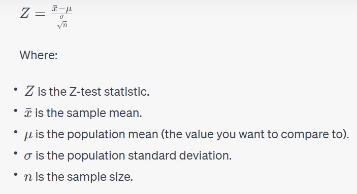
Purpose of the Z-Test: The primary purpose of a Z-test is to assess whether the sample mean (x̄) is significantly different from the population mean (μ) under the assumption that the population standard deviation (σ) is known. In other words, it helps us determine if the difference between the sample mean and the population mean is statistically significant or if it could have occurred due to random chance.
Formula for the Z-Test:
The Z-test statistic is calculated using the following formula:
Assumptions of the Z-Test: To use the Z-test effectively, several assumptions should be met:
- Random Sampling: The sample should be drawn randomly from the population to ensure it’s representative.
- Normal Distribution: The data should follow a normal distribution. While the central limit theorem allows for some deviation from normality when sample sizes are sufficiently large (typically, n > 30), a truly normal distribution is preferred.
- Independence: The data points in the sample should be independent of each other. This means that the value of one data point should not influence the value of another.
- Known Population Standard Deviation: The population standard deviation (σ) must be known. If it’s not known, you would typically use a t-test instead.
Steps to Conduct a Z-Test:
- Formulate Hypotheses:
- Null Hypothesis (H0): This is the default assumption that there is no significant difference between the sample mean and the population mean (H0: μ = μ0).
- Alternative Hypothesis (H1): This is the statement you’re testing, suggesting that there is a significant difference (H1: μ ≠ μ0 for a two-tailed test, or H1: μ > μ0 or H1: μ < μ0 for a one-tailed test).
- Select Significance Level (α): Choose the significance level, often denoted as α, which represents the probability of making a Type I error (rejecting the null hypothesis when it’s true). Common choices include α = 0.05 or α = 0.01.
- Collect Data and Calculate Sample Mean: Collect your sample data and calculate the sample mean (x̄) and the sample size (n).
- Calculate the Z-Test Statistic: Use the formula mentioned earlier to compute the Z-test statistic.
- Find Critical Values or P-Value: Depending on your alternative hypothesis, you can either find the critical values from a Z-table or calculate the p-value associated with your Z-test statistic.
- Make a Decision: If using critical values, compare your Z-test statistic to the critical values. If using a p-value, compare it to the chosen significance level (α).
- Draw a Conclusion: Based on the comparison, either reject the null hypothesis if the Z-test statistic falls in the critical region (or p-value is less than α) or fail to reject the null hypothesis if it falls in the non-critical region (or p-value is greater than α).
- Interpret the Result: If you reject the null hypothesis, you can conclude that there is a statistically significant difference between the sample mean and the population mean.
Common Use Cases: Z-tests are often used in quality control, marketing research, and medical research, among other fields, where the population standard deviation is known and sample sizes are relatively large. For instance, a manufacturer might use a Z-test to check if a new production process significantly changes the quality of their products compared to the known historical standard.
A Z-test is a powerful tool for assessing the significance of sample mean differences from a known population mean when certain assumptions are met. It helps in making data-driven decisions and drawing conclusions based on statistical evidence.
1.2 T-Test: A t-test is a statistical hypothesis test used to determine whether the means of two sets of data are significantly different from each other. It’s a valuable tool for comparing the means of two groups or samples and is particularly useful when dealing with small sample sizes. In this section, we cover the purpose of the t-test, its various types, assumptions, formulas, and steps to conduct the test.
Purpose of the T-Test: The t-test is used to assess whether there is a statistically significant difference between the means of two groups or samples. It helps researchers and analysts determine whether any observed difference is likely due to a real effect or simply a result of random variation. This can be applied to a wide range of scenarios, such as comparing the performance of two different treatments in a medical study, assessing the impact of an intervention, or determining if there’s a gender-based wage gap in an organization.
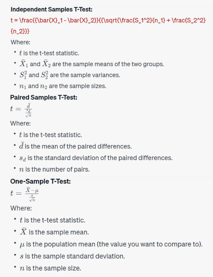
Types of T-Tests: There are several variations of the t-test, each designed for specific situations:
- Independent Samples T-Test: This t-test is used when you want to compare the means of two independent groups. For example, comparing the average test scores of students in two different schools.
- Paired Samples T-Test: In cases where the data is paired or matched, such as before-and-after measurements on the same subjects, a paired samples t-test is appropriate.
- One-Sample T-Test: When you want to compare the mean of a sample to a known population mean, you can use a one-sample t-test.
Formula for the T-Test: The formula for the t-test statistic depends on the type of t-test being conducted:
Assumptions of the T-Test: To use the t-test effectively, several assumptions should be met:
- Normality: The data within each group or sample should be approximately normally distributed. The Central Limit Theorem allows for some deviation from normality, especially with larger sample sizes.
- Independence: The data points within each group or sample should be independent of each other.
- Homogeneity of Variances: The variances within the groups should be roughly equal. However, there are variations of the t-test that can be used when this assumption is violated, such as Welch’s t-test.
Steps to Conduct a T-Test:
- Formulate Hypotheses:
- Null Hypothesis (H0): This is the default assumption that there is no significant difference between the two group means.
- Alternative Hypothesis (H1): This is the statement you’re testing, suggesting that there is a significant difference between the group means (H1: μ1 ≠ μ2 for a two-tailed test, or H1: μ1 > μ2 or H1: μ1 < μ2 for a one-tailed test).
- Select Significance Level (α): Choose the significance level, often denoted as α, which represents the probability of making a Type I error (rejecting the null hypothesis when it’s true). Common choices include α = 0.05 or α = 0.01.
- Collect Data and Calculate Sample Statistics: Collect your data and calculate the sample means, standard deviations, and sample sizes.
- Calculate the T-Test Statistic: Use the appropriate t-test formula to calculate the t-test statistic.
- Find Critical Values or P-Value: Depending on your alternative hypothesis, you can either find the critical values from a t-table or calculate the p-value associated with your t-test statistic.
- Make a Decision: If using critical values, compare your t-test statistic to the critical values. If using a p-value, compare it to the chosen significance level (α).
- Draw a Conclusion: Based on the comparison, either reject the null hypothesis if the t-test statistic falls in the critical region (or p-value is less than α) or fail to reject the null hypothesis if it falls in the non-critical region (or p-value is greater than α).
- Interpret the Result: If you reject the null hypothesis, you can conclude that there is a statistically significant difference between the two groups’ means.
Common Use Cases: T-tests are widely used in scientific research, social sciences, business analytics, and quality control to compare means between different groups or samples. They help determine if observed differences are statistically significant, allowing for data-driven decision-making.
The t-test is a versatile and powerful tool for comparing means in different situations, depending on the type of data and research question. It plays a crucial role in hypothesis testing, making it a fundamental concept in statistical analysis.
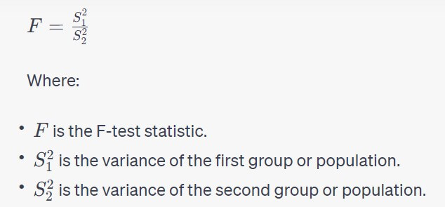
1.3 F-Test: The F-test, or Fisher’s F-test, is a statistical hypothesis test used to determine whether the variances of two or more groups or populations are significantly different. It is commonly used in analysis of variance (ANOVA) to assess if there are statistically significant differences between the variances of multiple groups. In this section, we cover the purpose of the F-test, its formula, assumptions, and steps to conduct the test.
Purpose of the F-Test: The primary purpose of the F-test is to compare the variances between two or more groups or populations. It helps researchers and analysts determine if there is a significant difference in variability among the groups. This test is often employed when you want to compare the performance, outcomes, or variations in several groups simultaneously.
Formula for the F-Test: The F-test statistic is calculated using the following formula:
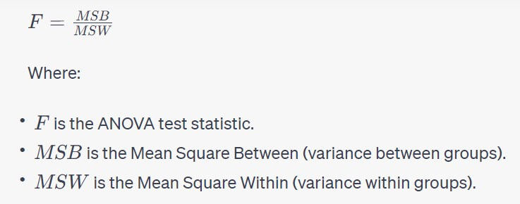
In the context of ANOVA, where you have more than two groups, the formula becomes more complex, involving the comparison of the mean squares (variances) between groups and within groups.
Assumptions of the F-Test: To use the F-test effectively, several assumptions should be met:
- Normality: The data within each group should be approximately normally distributed. Deviations from normality may be acceptable when sample sizes are sufficiently large, thanks to the Central Limit Theorem.
- Independence: The data points within each group should be independent of each other.
- Homogeneity of Variances (Homoscedasticity): This is a critical assumption for the F-test. It assumes that the variances within each group are roughly equal.
Steps to Conduct an F-Test:
- Formulate Hypotheses:
- Null Hypothesis (H0): This is the default assumption that there is no significant difference in variances between the groups.
- Alternative Hypothesis (H1): This is the statement you’re testing, suggesting that there is a significant difference in variances among the groups.
- Select Significance Level (α): Choose the significance level, often denoted as α, which represents the probability of making a Type I error (rejecting the null hypothesis when it’s true). Common choices include α = 0.05 or α = 0.01.
- Collect Data and Calculate Variances: Collect your data and calculate the variances of the groups or populations you want to compare.
- Calculate the F-Test Statistic: Use the formula mentioned earlier to compute the F-test statistic.
- Find Critical Values or P-Value: Depending on your alternative hypothesis, you can either find the critical values from an F-table or calculate the p-value associated with your F-test statistic.
- Make a Decision: If using critical values, compare your F-test statistic to the critical values. If using a p-value, compare it to the chosen significance level (α).
- Draw a Conclusion: Based on the comparison, either reject the null hypothesis if the F-test statistic falls in the critical region (or p-value is less than α) or fail to reject the null hypothesis if it falls in the non-critical region (or p-value is greater than α).
- Interpret the Result: If you reject the null hypothesis, you can conclude that there is a statistically significant difference in variances among the groups.
Common Use Cases: F-tests, especially in the context of ANOVA, are frequently used in experimental design, quality control, and scientific research. For example, in medical research, an F-test might be used to determine whether different drug treatments result in significantly different variances in patient outcomes.
The F-test is a valuable tool for comparing variances between groups, helping to identify significant differences in variability among the groups or populations. It plays a crucial role in statistical analysis and hypothesis testing when dealing with multiple categories or groups.
1.4 ANOVA (Analysis of Variance): Analysis of Variance, commonly referred to as ANOVA, is a powerful statistical technique used to determine whether there are statistically significant differences among the means of three or more groups. It is a fundamental tool for investigating the impact of categorical independent variables on a continuous dependent variable. In this section, we cover the purpose of ANOVA, its various types, assumptions, formulas, and steps to conduct the test.
Purpose of ANOVA: The primary purpose of ANOVA is to assess whether there are significant variations in group means when there are more than two groups. Instead of comparing each group pairwise, which can be cumbersome and lead to an increased likelihood of Type I errors, ANOVA allows you to compare means across all groups simultaneously. It helps researchers and analysts answer questions like:
- Is there a statistically significant difference in test scores among students from different schools?
- Does the type of fertilizer used significantly affect crop yields in multiple fields?
- Are there differences in the effectiveness of three different drug treatments on patient recovery times?
Types of ANOVA:
- One-Way ANOVA: This is the most basic form of ANOVA and is used when you have one categorical independent variable with three or more levels (groups). It tests for differences in means across the groups.
- Two-Way ANOVA: In a two-way ANOVA, you have two categorical independent variables. It assesses how these two factors interact to affect the dependent variable.
- Repeated Measures ANOVA: This type of ANOVA is used when the same subjects are used for each treatment or condition. It’s often employed in experimental designs where subjects are measured repeatedly over time.
- Multivariate Analysis of Variance (MANOVA): MANOVA is an extension of ANOVA and is used when there are multiple dependent variables. It assesses the impact of one or more independent variables on two or more dependent variables.
Formula for One-Way ANOVA: The formula for the One-Way ANOVA test statistic is based on comparing the variance between groups to the variance within groups. It can be expressed as:
Assumptions of ANOVA: To use ANOVA effectively, several assumptions should be met:
- Independence: The data points within each group should be independent of each other.
- Normality: The data within each group should be approximately normally distributed. Deviations from normality may be acceptable with larger sample sizes due to the Central Limit Theorem.
- Homogeneity of Variances (Homoscedasticity): This critical assumption assumes that the variances within each group are roughly equal.
- Random Sampling: The data should be collected through random sampling methods to ensure it’s representative of the population.
Steps to Conduct a One-Way ANOVA:
- Formulate Hypotheses:
- Null Hypothesis (H0): This is the default assumption that there is no significant difference in means among the groups.
- Alternative Hypothesis (H1): This is the statement you’re testing, suggesting that there is a significant difference in means among the groups.
- Select Significance Level (α): Choose the significance level, often denoted as α, which represents the probability of making a Type I error (rejecting the null hypothesis when it’s true). Common choices include α = 0.05 or α = 0.01.
- Collect Data and Calculate Group Statistics: Collect your data and calculate the sample means and sample variances for each group.
- Calculate the ANOVA Test Statistic (F): Use the ANOVA formula to calculate the test statistic.
- Find Critical Value or P-Value: Depending on your alternative hypothesis, you can either find the critical value from an F-table or calculate the p-value associated with the F-test statistic.
- Make a Decision: If using a critical value, compare your F-test statistic to the critical value. If using a p-value, compare it to the chosen significance level (α).
- Draw a Conclusion: Based on the comparison, either reject the null hypothesis if the F-test statistic falls in the critical region (or p-value is less than α) or fail to reject the null hypothesis if it falls in the non-critical region (or p-value is greater than α).
- Post-Hoc Tests (if necessary): If your ANOVA results are significant, you may want to perform post-hoc tests to determine which specific group means differ from each other. Common post-hoc tests include Tukey’s HSD, Bonferroni, and Scheffe tests.
Common Use Cases: ANOVA is widely used in various fields such as biology, psychology, education, economics, and many more. Some common applications include comparing the effects of different treatments, assessing the impact of factors on product quality, or evaluating the performance of groups in academic or business settings.
ANOVA is a fundamental statistical tool for comparing means among multiple groups. It simplifies the process of evaluating group differences and helps in making data-driven decisions and drawing conclusions based on statistical evidence.
1.5 Wilcoxon Signed-Rank Test: The Wilcoxon Signed-Rank Test, often referred to simply as the Wilcoxon test, is a non-parametric statistical hypothesis test used to assess whether the median of a paired data set is significantly different from a hypothesized median. It is a robust alternative to the paired t-test when the data doesn’t meet the assumptions of normality or when the data is measured on an ordinal scale. In this section, we cover the purpose of the Wilcoxon Signed-Rank Test, its assumptions, formula, and steps to conduct the test.
Purpose of the Wilcoxon Signed-Rank Test: The Wilcoxon Signed-Rank Test is used to determine whether there is a significant difference between two related groups when the data is not normally distributed or when the assumption of equal variances is violated. It is commonly employed in research scenarios where you have paired data, such as before-and-after measurements, or in cases where you want to compare two matched groups. For example, it could be used to evaluate the effectiveness of a new teaching method by comparing the test scores of students before and after the method is implemented.
Assumptions of the Wilcoxon Signed-Rank Test: The Wilcoxon Signed-Rank Test is a non-parametric test, which means it is less sensitive to the distribution of the data. However, there are still some assumptions:
- Matched Pairs: The test is suitable for paired or matched data. Each observation in one group should be paired with a corresponding observation in the other group.
- Continuous or Ordinal Data: The data should be continuous or ordinal. It should not be used for nominal data.
- Symmetric Distribution of Differences: The distribution of the differences between paired observations should be symmetric. This means that if you calculate the differences (subtractions) between the paired observations, their distribution should be roughly symmetric.
Steps to Conduct the Wilcoxon Signed-Rank Test:
- Formulate Hypotheses:
- Null Hypothesis (H0): This is the default assumption that there is no significant difference between the paired groups (the population median difference is zero).
- Alternative Hypothesis (H1): This is the statement you’re testing, suggesting that there is a significant difference in the paired groups (the population median difference is not zero).
- Select Significance Level (α): Choose the significance level, often denoted as α, which represents the probability of making a Type I error (rejecting the null hypothesis when it’s true). Common choices include α = 0.05 or α = 0.01.
- Collect Data and Calculate Differences: Collect your paired data and calculate the differences (subtractions) between the paired observations.
- Rank the Absolute Differences: Arrange the absolute differences in ascending order and assign a rank to each. Ties should be handled by giving them the average of the ranks they would have occupied.
- Calculate the Test Statistic (W): The test statistic W is calculated as the sum of the signed ranks. The sign of each rank corresponds to the sign of the original difference.
- Find the Critical Value or P-Value: Use the appropriate table of critical values for the Wilcoxon Signed-Rank Test or a statistical software package to find the critical value or calculate the p-value associated with the test statistic.
- Make a Decision: If using critical values, compare the test statistic W to the critical value. If using a p-value, compare it to the chosen significance level (α).
- Draw a Conclusion: Based on the comparison, either reject the null hypothesis if the test statistic falls in the critical region (or p-value is less than α) or fail to reject the null hypothesis if it falls in the non-critical region (or p-value is greater than α).
Common Use Cases: The Wilcoxon Signed-Rank Test is commonly used in various fields, including medical research (to assess the effectiveness of treatments), psychology (to compare pre- and post-intervention measurements), and social sciences (to evaluate the impact of programs or interventions). It is especially valuable when dealing with non-normally distributed data or ordinal data.
The Wilcoxon Signed-Rank Test is a robust and versatile statistical method for comparing paired data when the data doesn’t meet the assumptions of the paired t-test. It helps researchers make informed decisions and draw conclusions based on the analysis of related groups.
1.6 Mann-Whitney U Test: The Mann-Whitney U test, also known as the Wilcoxon rank-sum test, is a non-parametric statistical hypothesis test used to determine whether there are significant differences between two independent groups. It is commonly used when dealing with ordinal or continuous data that do not meet the assumptions of normality or when comparing two groups with unequal variances. In this section, we cover the purpose of the Mann-Whitney U test, its assumptions, formula, and steps to conduct the test.
Purpose of the Mann-Whitney U Test: The Mann-Whitney U test is used to assess whether there is a significant difference in central tendencies (medians) between two independent groups. It is often employed when you want to compare two groups, such as two treatments, two populations, or two samples, without assuming that the data is normally distributed. For example, it could be used to compare the effectiveness of two different medications in reducing pain levels among patients.
Assumptions of the Mann-Whitney U Test: The Mann-Whitney U test is a non-parametric test, which means it is less sensitive to the distribution of the data. However, it does have some assumptions:
- Independence: The data points in each group should be independent of each other. This means that the value of one data point should not influence the value of another.
- Continuous or Ordinal Data: The data should be either continuous or ordinal. It is not suitable for nominal data.
- Random Sampling: The data should be collected through random sampling methods to ensure it’s representative of the population.
Steps to Conduct the Mann-Whitney U Test:
- Formulate Hypotheses:
- Null Hypothesis (H0): This is the default assumption that there is no significant difference in central tendencies between the two groups.
- Alternative Hypothesis (H1): This is the statement you’re testing, suggesting that there is a significant difference in central tendencies between the two groups.
- Select Significance Level (α): Choose the significance level, often denoted as α, which represents the probability of making a Type I error (rejecting the null hypothesis when it’s true). Common choices include α = 0.05 or α = 0.01.
- Collect Data: Collect your data from the two independent groups.
- Combine Data: Combine the data from both groups and assign a rank to each observation, starting from the smallest value. Ties should be handled by giving them the average of the ranks they would have occupied.
- Calculate the U Statistic for Each Group: The U statistic for each group is the sum of the ranks for that group. You’ll have one U value for Group 1 and one U value for Group 2.
- Calculate the Smaller U Value: Compare the U statistics for the two groups and select the smaller one as U. The other U value is then n1 * n2 – U, where n1 and n2 are the sample sizes of the two groups.
- Find the Critical Value or P-Value: Use an appropriate table of critical values for the Mann-Whitney U test or a statistical software package to find the critical value or calculate the p-value associated with the U statistic.
- Make a Decision: If using a critical value, compare the U statistic to the critical value. If using a p-value, compare it to the chosen significance level (α).
- Draw a Conclusion: Based on the comparison, either reject the null hypothesis if the U statistic falls in the critical region (or p-value is less than α) or fail to reject the null hypothesis if it falls in the non-critical region (or p-value is greater than α).
Common Use Cases: The Mann-Whitney U test is widely used in various fields, including healthcare (comparing treatment outcomes), marketing (assessing the effectiveness of advertising campaigns), and social sciences (analyzing survey responses). It is especially valuable when dealing with non-normally distributed data or when comparing two groups with unequal variances.
The Mann-Whitney U test is a robust and versatile statistical method for comparing two independent groups when the data doesn’t meet the assumptions of the independent samples t-test. It helps researchers make data-driven decisions and draw conclusions based on the analysis of independent groups.
1.7 Kruskal-Wallis H Test: The Kruskal-Wallis H test, often referred to as simply the Kruskal-Wallis test, is a non-parametric statistical hypothesis test used to determine whether there are significant differences among the medians of three or more independent groups. It is an extension of the Mann-Whitney U test for comparing more than two groups. The Kruskal-Wallis test is used when the data doesn’t meet the assumptions of normality, and it is employed to assess whether there are statistically significant differences in the central tendencies of multiple independent groups. In this section, we cover the purpose of the Kruskal-Wallis H test, its assumptions, formula, and steps to conduct the test.
Purpose of the Kruskal-Wallis H Test: The Kruskal-Wallis test is used to determine whether there are significant differences among three or more independent groups when comparing ordinal or continuous data. It is often employed when you want to compare multiple groups, such as different treatments, different populations, or different samples, without making the assumption that the data is normally distributed. For example, it could be used to compare the effectiveness of three or more different teaching methods in improving students’ test scores.
Assumptions of the Kruskal-Wallis H Test: The Kruskal-Wallis test is a non-parametric test, which means it is less sensitive to the distribution of the data. However, it does have some assumptions:
- Independence: The data points in each group should be independent of each other. This means that the value of one data point should not influence the value of another.
- Continuous or Ordinal Data: The data should be either continuous or ordinal. It is not suitable for nominal data.
- Random Sampling: The data should be collected through random sampling methods to ensure it’s representative of the population.
Steps to Conduct the Kruskal-Wallis H Test:
- Formulate Hypotheses:
- Null Hypothesis (H0): This is the default assumption that there is no significant difference in central tendencies among the groups.
- Alternative Hypothesis (H1): This is the statement you’re testing, suggesting that there is a significant difference in central tendencies among the groups.
- Select Significance Level (α): Choose the significance level, often denoted as α, which represents the probability of making a Type I error (rejecting the null hypothesis when it’s true). Common choices include α = 0.05 or α = 0.01.
- Collect Data: Collect your data from the three or more independent groups.
- Combine Data and Rank Observations: Combine the data from all groups and assign a rank to each observation, starting from the smallest value. Ties should be handled by giving them the average of the ranks they would have occupied.
- Calculate the Kruskal-Wallis Test Statistic (H): The test statistic H is calculated based on the ranks of the observations. It is a measure of the degree of difference among the group medians.
- Find the Critical Value or P-Value: Use an appropriate table of critical values for the Kruskal-Wallis H test or a statistical software package to find the critical value or calculate the p-value associated with the test statistic.
- Make a Decision: If using a critical value, compare the test statistic H to the critical value. If using a p-value, compare it to the chosen significance level (α).
- Draw a Conclusion: Based on the comparison, either reject the null hypothesis if the test statistic falls in the critical region (or p-value is less than α) or fail to reject the null hypothesis if it falls in the non-critical region (or p-value is greater than α).
- Post-Hoc Tests (if necessary): If your Kruskal-Wallis results are significant, you may want to perform post-hoc tests to determine which specific group medians differ from each other. Common post-hoc tests include Dunn’s test or Conover’s test.
Common Use Cases: The Kruskal-Wallis test is widely used in various fields, including healthcare (comparing treatment outcomes among multiple groups), education (evaluating the effectiveness of different teaching methods), and social sciences (analyzing survey responses across multiple groups). It is especially valuable when dealing with non-normally distributed data or when comparing three or more independent groups.
The Kruskal-Wallis H test is a robust and versatile statistical method for comparing the central tendencies of multiple independent groups when the data doesn’t meet the assumptions of analysis of variance (ANOVA). It helps researchers make data-driven decisions and draw conclusions based on the analysis of multiple groups.
2. Regression Analysis:
Regression analysis is another important branch of inferential statistics that focuses on modeling relationships between variables. It is used to predict one variable (the dependent variable) based on one or more other variables (independent variables). There are different types of regression analysis, each suited for various data types and research questions.
2.1 Linear Regression: Linear regression is a fundamental statistical technique used to model the relationship between a dependent variable and one or more independent variables by fitting a linear equation to the observed data. It is widely employed in various fields, including economics, science, social sciences, and engineering, to analyze and predict the relationships between variables. In this section, we cover the purpose of linear regression, its types, assumptions, formulas, and steps to conduct the analysis.
Purpose of Linear Regression: The primary purpose of linear regression is to model the relationship between one or more independent variables (predictors) and a dependent variable (response). It aims to establish a linear equation that can be used for prediction, understanding the nature of the relationship, and making informed decisions based on data. Some common applications include predicting stock prices based on economic indicators, understanding the effect of advertising spending on sales, and modeling the relationship between temperature and ice cream sales.
Types of Linear Regression:
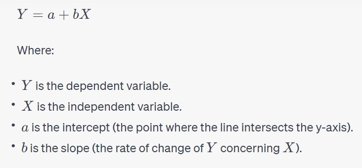
- Simple Linear Regression: In simple linear regression, there is only one independent variable used to predict the dependent variable. The equation for simple linear regression is typically represented as Y=a+bX where Y is the dependent variable, X is the independent variable, a is the intercept, and b is the slope.
- Multiple Linear Regression: Multiple linear regression involves two or more independent variables used to predict the dependent variable. The equation is an extension of simple linear regression and is represented as Y=a+b1X1+b2X2+⋯+bkXk where Y is the dependent variable, X1, X2, …, Xk are the independent variables, and a, b1, b2, …, bk are the coefficients.
- Polynomial Regression: Polynomial regression is used when the relationship between variables is nonlinear. It fits a polynomial equation to the data, such as , allowing for curved relationships.
- Logistic Regression: While logistic regression shares the name, it is used for categorical dependent variables, typically for binary classification problems. It models the probability of an event occurring.
Formula for Simple Linear Regression: The formula for simple linear regression can be expressed as:
The coefficients a and b are determined through the least squares method, which minimizes the sum of squared differences between the observed and predicted values of the dependent variable.
Assumptions of Linear Regression: To apply linear regression effectively, several assumptions should be met:
- Linearity: There should be a linear relationship between the independent variable(s) and the dependent variable.
- Independence: The observations should be independent of each other.
- Homoscedasticity: The variance of the errors (residuals) should be roughly constant across all levels of the independent variable(s).
- Normality of Residuals: The residuals (the differences between observed and predicted values) should be normally distributed.
- No or Little Multicollinearity: If multiple independent variables are used, they should not be highly correlated with each other.
Steps to Conduct Linear Regression:
- Formulate Hypotheses:
- Null Hypothesis (H0): The independent variable(s) do not significantly predict the dependent variable.
- Alternative Hypothesis (H1): The independent variable(s) significantly predict the dependent variable.
- Select Significance Level (α): Choose the significance level, often denoted as α, which represents the probability of making a Type I error (rejecting the null hypothesis when it’s true). Common choices include α = 0.05 or α = 0.01.
- Collect Data: Collect your data, which includes both the independent and dependent variables.
- Build the Regression Model: Fit the linear regression model to your data using appropriate software. This involves determining the coefficients (intercept and slopes) that minimize the sum of squared residuals.
- Assess the Model: Evaluate the goodness of fit, which includes examining the coefficients, R-squared (a measure of how well the model explains the variance), and assessing the assumptions of regression.
- Test Hypotheses: Use statistical tests or hypothesis testing to determine whether the independent variable(s) significantly predict the dependent variable.
- Make Predictions: Once the model is validated, use it to make predictions or infer relationships between variables.
- Interpret Results: Interpret the results, including the coefficients and their significance, to draw conclusions about the relationships between variables.
Common Use Cases: Linear regression is widely used in various fields for predictive modeling and understanding relationships between variables. It is frequently employed in financial forecasting, marketing analysis, scientific research, and social sciences. It helps in making predictions and data-driven decisions based on the analysis of the linear relationship between variables.
Linear regression is a versatile and widely used statistical technique for modeling and understanding the relationships between variables. It is a fundamental tool for data analysis and predictive modeling in various domains.
2.1 Logistic Regression: Logistic regression is a statistical method used for analyzing a dataset in which there are one or more independent variables that determine an outcome. The outcome is measured with a binary variable (in which there are only two possible outcomes), where the logistic regression model is used to analyze the relationship between the independent variables and the probability of a particular outcome occurring. In this section, we cover the purpose of logistic regression, its assumptions, formula, and steps to conduct the analysis.
Purpose of Logistic Regression: The primary purpose of logistic regression is to model the probability of a binary outcome, which can be expressed as either 0 or 1. It is widely used in various fields, including medicine (to predict the probability of a disease), finance (to assess the risk of an event happening), marketing (to predict whether a customer will buy a product), and more. Logistic regression provides a way to quantitatively examine the relationship between the dependent variable and one or more independent variables while accommodating the binary nature of the outcome.
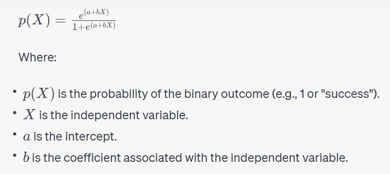
Formula for Logistic Regression: The logistic regression model uses the logistic function (sigmoid function) to model the relationship between the independent variables and the log-odds of the binary outcome. The logistic function is defined as:
The coefficients a and b are determined using a process called maximum likelihood estimation, which finds the values that maximize the likelihood of the observed data given the logistic function.
Assumptions of Logistic Regression: To apply logistic regression effectively, several assumptions should be met:
- Binary Outcome: The dependent variable must be binary, meaning it should have only two possible categories (e.g., 0 and 1, “yes” and “no,” “success” and “failure”).
- Independence of Observations: The observations should be independent of each other. In other words, the occurrence of an outcome for one observation should not influence the occurrence of an outcome for another observation.
- Linearity in Log-Odds: The relationship between the independent variables and the log-odds of the outcome should be linear.
- No or Little Multicollinearity: If multiple independent variables are used, they should not be highly correlated with each other, as high multicollinearity can affect the model’s stability.
Steps to Conduct Logistic Regression:
- Formulate Hypotheses:
- Null Hypothesis (H0): There is no significant relationship between the independent variable(s) and the probability of the binary outcome.
- Alternative Hypothesis (H1): There is a significant relationship between the independent variable(s) and the probability of the binary outcome.
- Select Significance Level (α): Choose the significance level, often denoted as α, which represents the probability of making a Type I error (rejecting the null hypothesis when it’s true). Common choices include α = 0.05 or α = 0.01.
- Collect Data: Collect your data, including the binary dependent variable and one or more independent variables.
- Build the Logistic Regression Model: Fit the logistic regression model to your data using appropriate software. This involves determining the coefficients (intercept and slopes) that maximize the likelihood of the observed data.
- Assess the Model: Evaluate the model’s fit, including examining the coefficients, assessing the assumptions, and conducting model diagnostics.
- Test Hypotheses: Use statistical tests or hypothesis testing to determine whether the independent variable(s) significantly predict the probability of the binary outcome.
- Make Predictions: Once the model is validated, use it to make predictions regarding the probability of the binary outcome based on the independent variables.
- Interpret Results: Interpret the results, including the coefficients and their significance, to draw conclusions about the relationship between the independent variables and the binary outcome.
Common Use Cases: Logistic regression is widely used for binary classification and predictive modeling in various fields. Common applications include disease diagnosis (e.g., predicting the presence or absence of a disease), credit risk assessment (e.g., predicting loan default), marketing (e.g., predicting customer churn), and more. It is a valuable tool for making informed decisions and drawing conclusions based on the analysis of binary outcomes.
Logistic regression is a powerful statistical technique for modeling and analyzing the relationship between independent variables and a binary outcome. It provides a probabilistic approach to binary classification and is an essential tool in the field of predictive modeling and data analysis.
2.3 Nominal Regression: Nominal regression, also known as multinomial logistic regression or categorical regression, is a statistical method used to model the relationship between a categorical dependent variable with three or more categories and one or more independent variables. It is an extension of logistic regression, specifically designed for situations where the dependent variable is nominal or categorical. In this section, we cover the purpose of nominal regression, its assumptions, formula, and steps to conduct the analysis.
Purpose of Nominal Regression: The primary purpose of nominal regression is to model the probability of an outcome belonging to one of several non-ordered categories or classes. This is particularly useful when the dependent variable is categorical with more than two categories. Nominal regression is widely used in various fields, including social sciences (to model political party choices), marketing (to analyze brand preferences), and healthcare (to predict patient diagnoses).
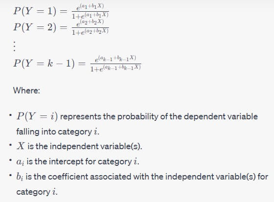
Formula for Nominal Regression: The formula for nominal regression involves modeling the probabilities of each category of the dependent variable using a set of equations. For a dependent variable with k categories, you have k−1 equations. Each equation corresponds to one category, and the last category is treated as the reference category. The model is typically represented as:
The coefficients are determined using maximum likelihood estimation to maximize the likelihood of the observed data given the model.
Assumptions of Nominal Regression: To apply nominal regression effectively, several assumptions should be met:
- Categorical Dependent Variable: The dependent variable should have three or more non-ordered categories.
- Independence of Observations: The observations should be independent of each other.
- Linearity in Log-Odds: The relationship between the independent variables and the log-odds of the outcome for each category should be linear.
- No Perfect Multicollinearity: The independent variables should not be perfectly correlated with each other, as this can lead to problems in estimating coefficients.
Steps to Conduct Nominal Regression:
- Formulate Hypotheses:
- Null Hypothesis (H0): There is no significant relationship between the independent variable(s) and the categories of the dependent variable.
- Alternative Hypothesis (H1): There is a significant relationship between the independent variable(s) and the categories of the dependent variable.
- Select Significance Level (α): Choose the significance level, often denoted as α, which represents the probability of making a Type I error (rejecting the null hypothesis when it’s true). Common choices include α = 0.05 or α = 0.01.
- Collect Data: Collect your data, including the categorical dependent variable and one or more independent variables.
- Build the Nominal Regression Model: Fit the nominal regression model to your data using appropriate software. This involves determining the coefficients (intercepts and slopes) that maximize the likelihood of the observed data.
- Assess the Model: Evaluate the model’s fit, including examining the coefficients, assessing the assumptions, and conducting model diagnostics.
- Test Hypotheses: Use statistical tests or hypothesis testing to determine whether the independent variable(s) significantly predict the categories of the dependent variable.
- Make Predictions: Once the model is validated, use it to make predictions regarding the probabilities of each category based on the independent variables.
- Interpret Results: Interpret the results, including the coefficients and their significance, to draw conclusions about the relationship between the independent variables and the categories of the dependent variable.
Common Use Cases: Nominal regression is used for modeling and analyzing categorical outcomes with three or more categories. It is applied in various fields, including market research (analyzing consumer preferences), social sciences (modeling political party choices), and healthcare (predicting disease diagnoses). It provides valuable insights into understanding and predicting categorical outcomes.
Nominal regression is a powerful statistical method for analyzing and modeling the relationship between categorical dependent variables with multiple categories and one or more independent variables. It is a fundamental tool for making informed decisions and drawing conclusions based on the analysis of categorical outcomes.
2.4 Ordinal Regression: Ordinal regression, also known as ordinal logistic regression or ordered logistic regression, is a statistical method used to model the relationship between an ordinal dependent variable (a variable with ordered categories) and one or more independent variables. It is an extension of logistic regression, specifically designed for situations where the dependent variable has ordered categories that are not evenly spaced. In this section, we cover the purpose of ordinal regression, its assumptions, formula, and steps to conduct the analysis.
Purpose of Ordinal Regression: The primary purpose of ordinal regression is to model the probability of an outcome belonging to one of several ordered categories or classes. Ordinal dependent variables have categories with a natural order but do not have evenly spaced intervals between categories. Ordinal regression is widely used in various fields, including psychology (to predict levels of satisfaction), education (to analyze student performance levels), and social sciences (to model responses to survey questions with ordered choices).
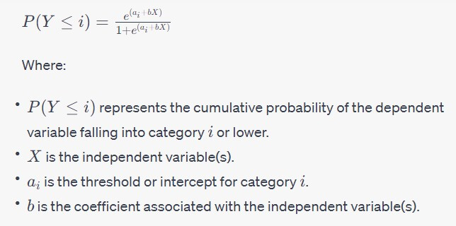
Formula for Ordinal Regression: The formula for ordinal regression involves modeling the probabilities of each category of the ordinal dependent variable using a set of equations. For a dependent variable with k ordered categories, you have k−1 equations. Each equation corresponds to one category, and the last category serves as the reference category. The model is typically represented as:
The coefficients are determined using maximum likelihood estimation to maximize the likelihood of the observed data given the model.
Assumptions of Ordinal Regression: To apply ordinal regression effectively, several assumptions should be met:
- Ordinal Dependent Variable: The dependent variable should have ordered categories with a clear, meaningful, and logical progression from one category to the next.
- Independence of Observations: The observations should be independent of each other.
- Proportional Odds Assumption: The proportional odds assumption states that the odds of moving from one category to a higher category are proportional to the odds of moving from any lower category to the current category. This assumption should be met, but if not, other ordinal regression models (e.g., partial proportional odds) can be considered.
- No Perfect Multicollinearity: The independent variables should not be perfectly correlated with each other, as high multicollinearity can affect the model’s stability.
Steps to Conduct Ordinal Regression:
- Formulate Hypotheses:
- Null Hypothesis (H0): There is no significant relationship between the independent variable(s) and the ordinal categories of the dependent variable.
- Alternative Hypothesis (H1): There is a significant relationship between the independent variable(s) and the ordinal categories of the dependent variable.
- Select Significance Level (α): Choose the significance level, often denoted as α, which represents the probability of making a Type I error (rejecting the null hypothesis when it’s true). Common choices include α = 0.05 or α = 0.01.
- Collect Data: Collect your data, including the ordinal dependent variable and one or more independent variables.
- Build the Ordinal Regression Model: Fit the ordinal regression model to your data using appropriate software. This involves determining the coefficients (thresholds and slopes) that maximize the likelihood of the observed data.
- Assess the Model: Evaluate the model’s fit, including examining the coefficients, assessing the assumptions, and conducting model diagnostics.
- Test Hypotheses: Use statistical tests or hypothesis testing to determine whether the independent variable(s) significantly predict the ordinal categories of the dependent variable.
- Make Predictions: Once the model is validated, use it to make predictions regarding the probabilities of each category based on the independent variables.
- Interpret Results: Interpret the results, including the coefficients and their significance, to draw conclusions about the relationship between the independent variables and the ordinal categories of the dependent variable.
Common Use Cases: Ordinal regression is used for modeling and analyzing ordinal outcomes with ordered categories. It is applied in various fields, including psychology (modeling responses on Likert scales), education (analyzing student performance levels), and marketing (predicting customer satisfaction levels). It provides valuable insights into understanding and predicting ordered categorical outcomes.
Ordinal regression is a powerful statistical method for analyzing and modeling the relationship between ordinal dependent variables with multiple ordered categories and one or more independent variables. It is a fundamental tool for making informed decisions and drawing conclusions based on the analysis of ordered categorical outcomes.
In conclusion, in the realm of inferential statistics, two powerful branches, hypothesis testing and regression analysis, play pivotal roles in unraveling the intricacies of data-driven decision-making. Hypothesis testing, comprised of various tests such as the Z-test, T-test, F-test, ANOVA, Wilcoxon signed-rank test, Mann-Whitney U test, and Kruskal-Wallis H test, allows researchers to scrutinize and validate their assumptions, drawing meaningful insights from sample data and often guiding them to accept or reject null hypotheses. On the other hand, regression analysis, spanning from linear and logistic regression to nominal and ordinal regression, equips analysts with the means to model relationships, predict outcomes, and understand the influences of multiple independent variables on a dependent variable. These techniques, underpinned by assumptions and statistical rigor, empower professionals in diverse fields, from healthcare to marketing, to harness the power of data for informed decision-making. In a data-centric world, the synergy between hypothesis testing and regression analysis provides a robust foundation for drawing actionable conclusions and shaping the landscape of modern research and decision science.
References:
- Agresti, A., & Finlay, B. (2018). “Statistical Methods for the Social Sciences.” Pearson.
- Berenson, M. L., Levine, D. M., & Szabat, K. A. (2015). “Basic Business Statistics: Concepts and Applications.” Pearson.
- Bryman, A. (2015). “Social Research Methods.” Oxford University Press.
- Hulley, S. B., Cummings, S. R., Browner, W. S., Grady, D. G., & Newman, T. B. (2013). “Designing Clinical Research.” Lippincott Williams & Wilkins.
- Keller, G. (2013). “Statistics for Management and Economics.” Cengage Learning.
- McKinney, W. (2018). “Python for Data Analysis.” O’Reilly Media.
- Moore, D. S., McCabe, G. P., & Craig, B. A. (2016). “Introduction to the Practice of Statistics.” W. H. Freeman.
- OpenStax College. (2014). “Introductory Statistics.” OpenStax CNX. Retrieved from https://cnx.org/contents/7a0f20e8-b5e3-4860-a2f8-62af7ca0f70e@2
- Trochim, W. M. K., & Donnelly, J. P. (2008). “Research Methods: The Essential Knowledge Base.” Cengage Learning.
- VanderPlas, J. (2016). “Python Data Science Handbook.” O’Reilly Media.

Library Lecturer at Nurul Amin Degree College

